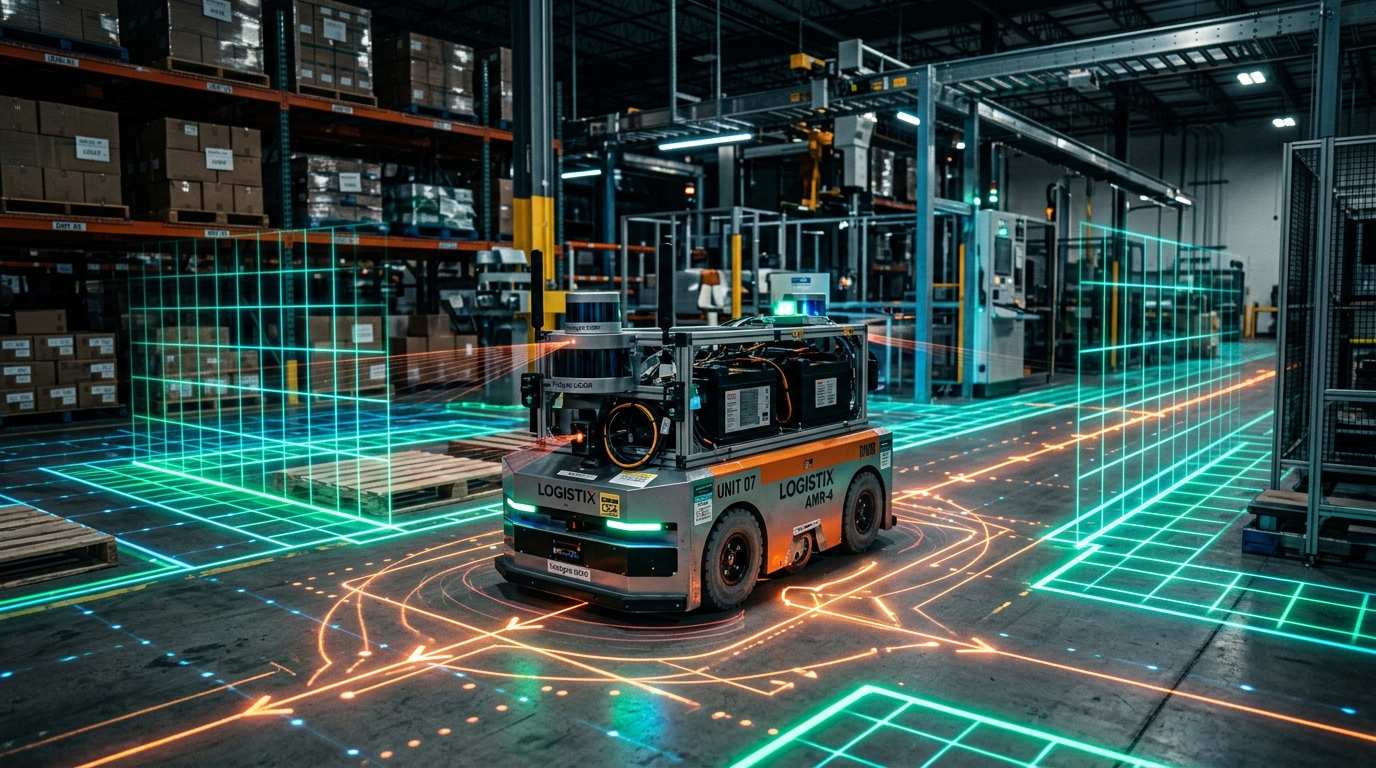
Autonomous Navigation & Path Planning: Global, Local Planners & Nav2 Costmaps Explained

Core Engineering Takeaways

•Navigation separates into two loops: a slow Global Planner (1-5 Hz) finding topological paths, and a fast Local Controller (20-100 Hz) steering clear of dynamic obstacles.
•A* achieves optimal heuristic graph search, whereas RRT* (Rapidly-exploring Random Trees) explores high-degree-of-freedom continuous configuration spaces with asymptotic optimality.
•The Timed Elastic Band (TEB) planner deforms the global path in real time, optimizing for time-of-flight, clearance distance, and motor acceleration limits simultaneously.
•Costmaps convert raw sensor point clouds into 2D/3D grids with lethal obstacle zones and exponential inflation decays so robots never clip walls.
•Modern ROS 2 Nav2 uses Behavior Trees (BT) instead of finite state machines, allowing clean recovery behaviors (backing up, spinning, clearing costmaps) without code lockups.

Prerequisites

Coordinate frames and transform tree (TF2) basics
Differential drive and unicycle kinematics
Basic probability and grid representations (occupancy grids)

1. The Navigation Stack Architecture: Global vs Local Planning

A common rookie mistake is attempting to steer a robot directly along an A* shortest path. A raw geometric path consists of sharp corners that violate physical motor dynamics and ignores people walking in front of the robot.

Modern robotics decouples motion planning into a hierarchical two-tier control architecture:

1
Global Planner (Macro-scale): Runs on a static map (SLAM occupancy grid) at 1–5 Hz. It computes an obstacle-free geometric backbone between the robot's current pose and the destination goal coordinate $(x, y, \theta)$ .
2
Local Controller / Trajectory Generator (Micro-scale): Runs at 20–50 Hz using live real-time sensor streams (LiDAR scans, depth camera point clouds). It generates smooth velocity commands $(v_x, v_y, \omega)$ that steer around dynamic obstacles while keeping close to the global backbone.

Why Two Loops?

Calculating a complete 50-meter floor path at 50 Hz would melt your CPU. Computing a global topological path once (or every few seconds) and allowing a lightweight local planner to handle split-second pedestrian avoidance is the standard industrial pattern.

2. Global Path Planning: Graph Search (A, Dijkstra) & Sampling (RRT)

Global planners compute paths through a configuration space (C-space) where the robot is represented as a dimensionless point and obstacles are grown by the robot's inscribed radius.

Graph-Based Planners: Dijkstra vs A*

Dijkstra's Algorithm: Uniformly expands outward in concentric rings, evaluating cost $g(n)$ from the start node. It guarantees the shortest path but evaluates unnecessary nodes away from the goal.
A* Algorithm: Uses a heuristic $h(n)$ (typically Euclidean or Manhattan distance) to prioritize exploration towards the goal node:

f(n) = g(n) + h(n)

where $g(n)$ is the accumulated path cost from start to node $n$ , and $h(n)$ is the estimated remaining distance to the goal.

Sampling-Based Planners: RRT and RRT*

In large outdoor spaces or high-dimensional manipulator arms, grid search suffers from the "curse of dimensionality". RRT (Rapidly-exploring Random Trees) incrementally builds a search tree by picking random points in continuous space. RRT* introduces local edge rewiring: when a new node is added, it rewires neighboring nodes if passing through the new node yields lower accumulated path cost, guaranteeing asymptotic optimality.

A* Heuristic Evaluation Function

f(n) = g(n) + \epsilon \cdot \sqrt{(x_g - x_n)^2 + (y_g - y_n)^2}

In Simple Words: The total estimated path cost f(n) balances past path travel cost g(n) with estimated straight-line Euclidean distance to the goal.

Variables Breakdown:

g(n)

Actual cumulative cost from start position to current cell nUnit: Cost units

h(n)

Heuristic estimated Euclidean distance from n to goal (x_g, y_g)Unit: Meters

\epsilon

Heuristic weight factor (\epsilon = 1 is standard A*; \epsilon > 1 is greedy weighted A*)

Table 1: Global Path Planning Algorithms Compared

Algorithm	Search Paradigm	Optimality	CPU Cost	Best Suited For
Dijkstra	Graph Grid (Exhaustive)	Guaranteed Shortest	High (Explores all directions)	Pre-computed static transit routes
A*	Graph Grid (Heuristic)	Guaranteed Shortest (if h admissible)	Moderate	2D Indoor Warehouses and AGVs
RRT	Continuous Sampling	Sub-optimal (Probabilistically Complete)	Low / Fast	Quick feasibility checks in mazes
RRT*	Continuous Sampling + Rewiring	Asymptotically Optimal	Moderate-High	High-DOF arms and off-road navigation
Theta*	Any-Angle Grid Search	Near-Optimal (Straight diagonals)	Moderate	Robots that do not want jagged 90° zig-zags

3. Local Trajectory Controllers: DWB, TEB & Model Predictive Control (MPC)

The local controller takes the global path and generates actuator velocity commands $(v, \omega)$ every 20–50 ms.

1. DWA / DWB (Dynamic Window Approach)

Discretizes the robot's velocity space into allowable $(v, \omega)$ pairs based on current motor accelerations over a brief time window $\Delta t$ . It forward-simulates circular trajectory arcs, scores them against obstacle clearance, global path alignment, and forward speed, and picks the highest scoring velocity tuple.

2. TEB (Timed Elastic Band)

Represents the path as an elastic rubber band deformed by virtual forces:

Internal elastic tension pulling nodes together (shortening time).
Repulsive potential fields pushing nodes away from live LiDAR obstacles.
Non-holonomic kinematic constraints preventing sideways wheel slippage.

TEB optimizes both spatial waypoints and time intervals $\Delta T_i$ simultaneously, producing buttery-smooth trajectories that brake naturally before corners.

3. MPC (Model Predictive Control)

Uses a physics-based dynamic model of the vehicle to solve a quadratic optimization problem over a finite preview horizon $N$ (e.g., 20 steps into the future). Highly popular in autonomous highway vehicles and high-speed Ackermann rovers.

simple_dwb_sample.py

python

import numpy as np

def evaluate_trajectory_velocity(v, w, dt, horizon, obstacles, goal_pose):
    """
    Simulates unicycle trajectory: x_{t+1} = x_t + v*cos(theta)*dt
    Scores for clearance, speed, and goal distance.
    """
    x, y, theta = 0.0, 0.0, 0.0
    min_dist_to_obs = float('inf')
    
    for t in np.arange(0, horizon, dt):
        x += v * np.cos(theta) * dt
        y += v * np.sin(theta) * dt
        theta += w * dt
        
        # Calculate distance to nearest obstacle point
        for ox, oy in obstacles:
            dist = np.hypot(x - ox, y - oy)
            if dist < min_dist_to_obs:
                min_dist_to_obs = dist
                
    if min_dist_to_obs < 0.25: # Collision threshold (inscribed radius)
        return -1.0 # Lethal collision
        
    dist_to_goal = np.hypot(goal_pose[0] - x, goal_pose[1] - y)
    score = (0.6 * v) + (0.3 * min_dist_to_obs) - (0.5 * dist_to_goal)
    return score

Note: Core evaluation function of Dynamic Window local planning: forward-simulating motion arcs and scoring against obstacle clearance and goal heading.

4. Costmaps: Static, Obstacle, Voxel & Inflation Decay Math

A costmap translates geometric surroundings into a 2D grid of 8-bit cost values from 0 (Free Space) to 255 (Lethal Obstacle).

Modern Nav2 costmaps use a layered plugin pipeline:

Static Map Layer: Reads the SLAM 2D occupancy grid (walls, permanent pillars).
Obstacle Layer: Integrates live 2D planar LiDAR scans via raytracing (marking hits as obstacles and clearing free space along laser rays).
Voxel Layer: Maintains 3D voxel columns from RGB-D depth cameras to detect low obstacles (pallets, steps) and overhead overhangs (pipes).
Inflation Layer: Propagates costs outwards from lethal boundaries using an exponential decay function. This guarantees the robot's physical bumper never touches an obstacle.

Costmap Inflation Decay Formula

Cost(d) = 253 \cdot \exp(-k_{decay} \cdot (d - r_{inscribed}))

In Simple Words: Beyond the robot inscribed radius r_inscribed (lethal zone), costs fall off exponentially with distance d until reaching zero at inflation radius.

Variables Breakdown:

Cost(d)

Cost value assigned to grid cell at distance dUnit: 0 to 254

r_{inscribed}

Inscribed circle radius of the robot footprintUnit: Meters

k_{decay}

Cost scaling factor (higher values create steep, narrow safety bands)Unit: m^{-1}

d

Euclidean distance from grid cell to nearest lethal obstacleUnit: Meters

5. Kinematics & Dynamic Feasibility: Differential vs Ackermann vs Omnidirectional

Path planners must know what motion the chassis can physically execute:

1
Holonomic (Omnidirectional / Mecanum):

Degrees of freedom match controllable inputs: can drive sideways $(v_y \neq 0)$ while rotating $(\omega \neq 0)$ .
Simplest for path planning; any $(x, y)$ coordinate can be traversed directly.

2
Non-Holonomic Differential Drive (2-Wheel / Unicycle):

Cannot translate sideways ( $v_y = 0$ ). Must rotate in place before driving forward.
Requires trajectories with continuous curvature or explicit zero-radius pivot points.

3
Non-Holonomic Ackermann Steering (Car-like):

Cannot rotate in place! Has a minimum turning radius $R_{min} = \frac{L}{\tan(\delta_{max})}$ .
Must use specialized planners like Hybrid A* or Reeds-Shepp curves that account for reverse gearing and steering angle limits.

Table 2: Robot Kinematic Drive Types in Motion Planning

Drive Architecture	Sideways Translation	In-Place Rotation	Minimum Turning Radius	Standard Local Planner
Differential Drive (2WD/Tracks)	No (v_y = 0)	Yes (Zero radius)	0 meters	DWB, TEB Local Planner
Ackermann (Car steering)	No (v_y = 0)	No	L / tan(delta_max)	TEB (Ackermann mode), Hybrid A*, MPC
Mecanum / Omnidirectional	Yes (Full holonomic)	Yes (Simultaneous)	0 meters	Omni DWB, MPPI, Vector Pursuit
Tricycle / Steered Wheel	No	No	Varies by pivot angle	Pure Pursuit, TEB

6. Nav2 Behavior Trees: Execution Flows & Recovery Strategies

In early ROS 1 Navigation (move_base), navigation was managed by hardcoded C++ state machines. When a robot encountered an unexpected obstacle, it frequently got trapped in infinite recovery spin loops.

ROS 2 Nav2 replaces state machines with Behavior Trees (BT):

Control Nodes: Sequence (AND), Fallback/Selector (OR), and Parallel nodes.
Action Nodes: ComputePathToPose (Global), FollowPath (Local), BackUp, Spin, ClearEntireCostmap.
Condition Nodes: IsStuck, IsGoalReached, TransformAvailable.

If the Local Planner reports that no collision-free trajectory exists for 3 consecutive iterations, the Behavior Tree fallback branch automatically triggers:

1
Clear Costmap Layer (purge phantom sensor artifacts).
2
Back Up 20 cm (retreat out of tight pinch-point).
3
Spin 360° (refresh LiDAR surroundings).
4
Re-compute Global Path from current pose.

nav2_behavior_tree.xml

xml

<root main_tree_to_execute="MainTree">
  <BehaviorTree ID="MainTree">
    <RecoveryNode number_of_retries="4" name="NavigateRecovery">
      <PipelineSequence name="NavigateWithReplanning">
        <RateController hz="1.0">
          <ComputePathToPose goal="{goal}" path="{path}" planner_id="GridBased"/>
        </RateController>
        <FollowPath path="{path}" controller_id="FollowPath"/>
      </PipelineSequence>
      <ReactiveFallback name="RecoveryFallback">
        <GoalUpdated/>
        <RoundRobin name="RecoveryActions">
          <ClearEntireCostmap name="ClearCostmap" service_name="local_costmap/clear_entirely_local_costmap"/>
          <Spin spin_dist="1.57" name="SpinRecovery"/>
          <Wait wait_duration="3" name="WaitRecovery"/>
          <BackUp backup_dist="0.25" backup_speed="0.08" name="BackupRecovery"/>
        </RoundRobin>
      </ReactiveFallback>
    </RecoveryNode>
  </BehaviorTree>
</root>

Note: ROS 2 Nav2 Behavior Tree showing pipeline sequence of global re-planning and reactive fallback recovery behaviors (Costmap clearing, Spin, Wait, Back Up).

Frequently Asked Questions

Common Questions & Troubleshooting

Q:Why does my robot oscillate back and forth when approaching the goal pose?

This classic "hunting" oscillation happens when the goal XY tolerance is set too tight (e.g. 2 cm) while odometry drift or noise is 3-5 cm. Fix this by: (1) Increasing xy_goal_tolerance to 0.08–0.15 m, (2) Enabling yaw_goal_tolerance latching so the robot stops translating before rotating to final heading, and (3) Decreasing deceleration limits near the goal.

Q:What is the difference between Inscribed Radius and Circumscribed Radius?

Inscribed Radius is the radius of the largest circle entirely inside your robot footprint. Any obstacle inside this radius is guaranteed to be a collision. Circumscribed Radius is the radius of the smallest circle containing your entire footprint (including corners). If an obstacle is farther than the circumscribed radius, the robot can rotate freely without hitting anything.

Q:When should I choose TEB over DWB in ROS 2 Nav2?

Use DWB for simple, circular differential drive robots in wide indoor spaces where low CPU usage is critical. Choose TEB when: (1) Your robot is non-circular (rectangular or long pallet mover), (2) You have an Ackermann car chassis with turning radius limits, or (3) You navigate tight corridors with dynamic obstacles where velocity and acceleration constraints must be optimized simultaneously.

Previous ArticleEdge AI for Robotics: CPUs, GPUs, NPUs & On-Device Inference Explained Next ArticleLiDAR Sensors & 3D Point Cloud Processing: ToF Physics, PCL, Voxel Grids & ICP