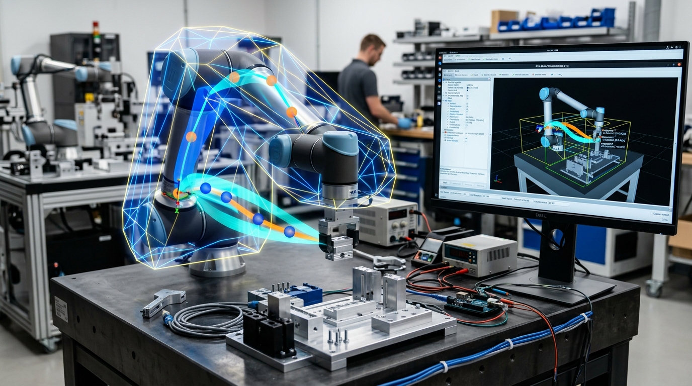
Robot Arm Motion Planning with MoveIt 2: Kinematics, Collision Checking & OMPL | Knowledge Hub

Core Engineering Takeaways

•Motion planning for serial manipulators takes place in Configuration Space (C-Space), where each dimension represents an independent joint angle $\theta_i$, transforming complex 3D link collision boundaries into C-Space obstacle manifolds.
•Standard numerical IK solvers (like KDL) frequently get trapped in local singularities; production systems use TRAC-IK (dual SQP + genetic optimizer) or analytical IKFast solutions that execute in microseconds.
•Collision checking accounts for up to 90% of total motion planning compute time; MoveIt 2 utilizes FCL (Flexible Collision Library) bounding volume hierarchies (OBBs and AABBs) to prune millions of non-colliding link-obstacle tests.
•OMPL sampling algorithms find geometric paths through high-dimensional C-space, but the resulting waypoints have no time or velocity information until processed by a time-optimal parameterizer like TOPP-RA.
•Pilz Industrial Motion Generator provides deterministic linear (LIN), point-to-point (PTP), and circular (CIRC) trajectories essential for machine tending and welding where predictable Cartesian paths are mandatory.

Prerequisites

Forward and Inverse Kinematics fundamentals (DH parameters, Jacobian matrices)
Basic ROS 2 concepts (Nodes, Actions, Parameters, Launch files)
URDF/Xacro robot description models and TF2 transform tree

1. The Motion Planning Pipeline: From Cartesian Goals to Motor Torques

Planning motion for a 6-DoF or 7-DoF articulated robot arm is vastly more mathematically intricate than navigating a 2D mobile robot base on a floor.

A mobile robot moves in $SE(2)$ with 3 degrees of freedom. A 6-axis articulated manipulator operates with 6 rotary joints, where each joint angle $\theta_i \in [-\pi, +\pi]$ influences the spatial position of every subsequent link in the kinematic chain.

The 5 Stages of the MoveIt 2 Motion Pipeline:

1
Goal Specification: A target end-effector pose $\mathbf{T}_{target} \in SE(3)$ or specific joint configuration is received.
2
Kinematic Inversion: An IK solver computes valid joint configurations $\mathbf{q} \in \mathbb{R}^n$ reaching the target pose without violating joint physical limits.
3
C-Space Path Planning: OMPL algorithms (such as RRT-Connect) explore the free Configuration Space ( $C_{free}$ ) to find a collision-free geometric path connecting start pose $\mathbf{q}_{start}$ to goal $\mathbf{q}_{goal}$ .
4
Time Parameterization: The geometric polyline is smoothed into a continuous trajectory ( $C^2$ continuous splines) respecting joint velocity limits $\mathbf{v}_{max}$ and joint acceleration limits $\mathbf{a}_{max}$ .
5
Controller Execution: The trajectory is dispatched via ROS 2 FollowJointTrajectory actions to low-level motor servo drives.

Why Plan in C-Space?

In Cartesian 3D workspace, the robot links are complex polyhedral meshes moving and rotating relative to each other. In Configuration Space (C-Space), the entire robot collapses into a single infinitesimal point $\mathbf{q} = (\theta_1, \theta_2, \dots, \theta_n)$ moving through an n-dimensional space.

2. Inverse Kinematics Engines: TRAC-IK, KDL, bio_ik & Analytical IKFast

Given a desired 6D pose of the robot gripper $[X, Y, Z, \text{Roll}, \text{Pitch}, \text{Yaw}]^T$ , the Inverse Kinematics (IK) solver must compute the corresponding joint angles $\mathbf{q} = [\theta_1, \dots, \theta_6]^T$ .

Primary IK Solver Families:

1
Numerical Newton-Raphson / KDL (Kinematics and Dynamics Library):

Uses the pseudoinverse or damped least squares of the manipulator Jacobian matrix:

\Delta \mathbf{q} = \mathbf{J}^T (\mathbf{J}\mathbf{J}^T + \lambda^2 \mathbf{I})^{-1} \Delta \mathbf{x}

Flaw: Easily becomes trapped in local kinematic minima or singularities (wrist alignment), failing on up to 20% of valid physical poses.

2
TRAC-IK (Dual Solver Engine):

Runs two parallel concurrent threads: an augmented numerical Jacobian solver and a global Sequential Quadratic Programming (SQP) optimizer.
Whichever thread converges first returns the solution.
Achieves $> 99.5\%$ success rate across full workspace reach.

3
Analytical IKFast (OpenRAVE):

Derives exact closed-form algebraic equations for robots satisfying the Pieper Criterion (three consecutive intersecting revolute axes, typical of universal industrial 6-axis arms like KUKA, FANUC, UR).
Computes all 8 mathematical IK solutions in less than 4 microseconds with zero local minima issues.

Table 1: Manipulator Inverse Kinematics Solver Shootout

Solver	Type	Solve Time	Success Rate	Redundancy (7-DoF)
KDL	Numerical Jacobian	1.5 - 5.0 ms	~80 - 85%	Poor
TRAC-IK	Dual Numerical + SQP	0.2 - 0.8 ms	> 99.5%	Excellent
bio_ik	Memetic Genetic Algorithm	0.5 - 2.0 ms	> 99.8%	Superb (Multi-goal optimization)
IKFast	Analytical Closed-Form	< 0.005 ms (5 μs)	100% (within envelope)	Requires parameterized null-space

3. Planning Scene Monitors & 3D Collision Detection: FCL & OctoMap

A path is useless if the robot forearm smashes into a table leg or pinches against an adjacent workcell wall.

MoveIt 2 maintains a live Planning Scene Monitor that fuses:

Self-Collision Matrix (ACM): A precomputed lookup table disabling checks between links that are physically adjacent or mechanically incapable of colliding, saving huge computational overhead.
Static Scene Meshes: CAD models of conveyor belts, tables, safety cages, and fixtures represented as triangular meshes.
Dynamic Sensor Point Clouds (OctoMap): 3D voxels generated from real-time RealSense or LiDAR depth frames.

Continuous Collision Checking with FCL (Flexible Collision Library)

Discrete collision checks only verify whether link positions at time $t$ intersect an obstacle. If the robot moves rapidly between $t$ and $t + \Delta t$ , it could tunnel directly through a thin obstacle (the "bullet tunneling effect").

Continuous collision checking sweeps the geometric envelope of each link over the trajectory segment, guaranteeing zero penetration.

Allowed Collision Matrix (ACM) Tuning

Always generate a customized Allowed Collision Matrix during MoveIt Setup Assistant configuration. By disabling collision tests between adjacent links and permanently clear link pairs, you reduce collision checking CPU time by 60–80%.

4. Path Planning in C-Space: OMPL RRT-Connect, PRM* & TrajOpt

The Open Motion Planning Library (OMPL) provides the core path generation engine for MoveIt 2.

1. RRT-Connect (Rapidly-exploring Random Trees - Connect)

The universal default for point-to-point manipulator planning.
Grows two trees simultaneously: one rooted at the start state $\mathbf{q}_{start}$ and one rooted at the goal state $\mathbf{q}_{goal}$ .
Each tree randomly samples C-Space points and extends branches toward the other.
Extremely fast at finding an initial valid path through cluttered obstacle scenes, but generates rough, jagged trajectories requiring post-process shortcut smoothing.

2. PRM* (Probabilistic Roadmap Star)

A multi-query planning approach.
Builds a permanent graph of collision-free nodes throughout the robot workcell during idle time.
When an execution request arrives, it instantly connects start and goal to the nearest roadmap nodes using Dijkstra or A*.
Ideal for assembly lines where the obstacles are static and millions of pick-and-place cycles repeat daily.

3. Trajectory Optimization (TrajOpt & STOMP)

Instead of randomized sampling, treats motion planning as a continuous non-linear optimization problem.
Minimizes trajectory length and joint accelerations subject to signed distance field (SDF) clearance penalties.

OMPL Path Straightening Shortcut Optimization

\mathbf{q}(\alpha) = (1 - \alpha) \mathbf{q}_a + \alpha \mathbf{q}_b, \quad \alpha \in [0, 1]

In Simple Words: The path simplifier iteratively picks two non-adjacent waypoints on the jagged RRT path and checks if a straight C-Space line between them is collision-free. If clear, all intermediate zig-zag waypoints are pruned.

Variables Breakdown:

\mathbf{q}_a

Upstream waypoint in joint configuration space

\mathbf{q}_b

Downstream waypoint in joint configuration space

\alpha

Interpolation scalar along the segment

Worked Example:

Prunes a raw 48-waypoint RRT-Connect path down to 6 smooth, straight C-Space transitions in under 8 milliseconds.

5. Time Parameterization: TOPP-RA vs Iterative Parabolic Splines

Sampling-based algorithms output pure geometric path coordinates $[\mathbf{q}_0, \mathbf{q}_1, \dots, \mathbf{q}_m]$ without timestamps. Feeding these directly to motor drives would command infinite acceleration and trip servo overcurrent faults.

Time parameterization assigns timestamps, velocities $\dot{\mathbf{q}}(t)$ , and accelerations $\ddot{\mathbf{q}}(t)$ along the path.

1. Iterative Parabolic Time Parameterization (IPTP)

The legacy MoveIt 1 default.
Fits trapezoidal acceleration profiles along path segments.
Suffers from numeric stability issues when waypoints are closely spaced, frequently causing velocity oscillations near path endpoints.

2. TOPP-RA (Time-Optimal Path Parameterization based on Reachability Analysis)

The state-of-the-art default in MoveIt 2.
Formulates the timing problem as linear programming on path reachability sets.
Pushes robot joints to their exact physical torque and velocity boundaries without violating jerk constraints.
Up to 35% faster cycle times on identical geometric paths compared to legacy parabolic timing!

Joint Kinematic Constraint Boundary

|\dot{q}_i(t)| \le v_{max, i}, \quad |\ddot{q}_i(t)| \le a_{max, i}, \quad |\dddot{q}_i(t)| \le j_{max, i}

In Simple Words: The time parameterization algorithm must strictly constrain joint velocities, accelerations, and jerk derivatives beneath factory motor limits at every millisecond of the motion.

Variables Breakdown:

v_{max, i}

Maximum allowable velocity for joint iUnit: rad/s

a_{max, i}

Maximum allowable acceleration for joint iUnit: rad/s²

j_{max, i}

Maximum allowable jerk for joint iUnit: rad/s³

Worked Example:

A UR5e elbow joint rated for 3.14 rad/s and 10 rad/s² is kept strictly within limits while maximizing travel speed along the trajectory.

6. Production Implementation: MoveIt 2 MoveGroupInterface & Pilz Motions

The primary programming interface for application developers in ROS 2 is the modern C++ moveit::planning_interface::MoveGroupInterface.

Below is a robust production C++ implementation demonstrating target pose planning, speed scaling, and execution with error handling:

arm_trajectory_planner_node.cpp

cpp

#include <rclcpp/rclcpp.hpp>
#include <geometry_msgs/msg/pose_stamped.hpp>
#include <moveit/move_group_interface/move_group_interface.h>

class ArmPlanningService : public rclcpp::Node {
public:
  ArmPlanningService(const rclcpp::NodeOptions& options)
      : Node("arm_planning_service", options) {}

  void plan_and_execute_pick() {
    // 1. Initialize MoveGroup for the "manipulator" arm planning group
    auto move_group = moveit::planning_interface::MoveGroupInterface(
        shared_from_this(), "manipulator");

    // 2. Set strict kinematic limits for safety (50% max speed)
    move_group.setMaxVelocityScalingFactor(0.5);
    move_group.setMaxAccelerationScalingFactor(0.5);
    move_group.setPlanningTime(5.0);
    move_group.setPlannerId("RRTConnectkConfigDefault");

    // 3. Define the desired Cartesian Target Pose (in world/base frame)
    geometry_msgs::msg::PoseStamped target_pose;
    target_pose.header.frame_id = "base_link";
    target_pose.pose.position.x = 0.45;
    target_pose.pose.position.y = 0.15;
    target_pose.pose.position.z = 0.35;
    // Orientation: End-effector pointing downward (-Z)
    target_pose.pose.orientation.x = 0.0;
    target_pose.pose.orientation.y = 1.0;
    target_pose.pose.orientation.z = 0.0;
    target_pose.pose.orientation.w = 0.0;

    move_group.setPoseTarget(target_pose);

    // 4. Compute the Motion Plan
    moveit::planning_interface::MoveGroupInterface::Plan planned_trajectory;
    auto success = (move_group.plan(planned_trajectory) == 
                    moveit::core::MoveItErrorCode::SUCCESS);

    if (success) {
      RCLCPP_INFO(this->get_logger(), 
        "Plan computed successfully with %zu trajectory waypoints. Executing...",
        planned_trajectory.trajectory_.joint_trajectory.points.size());

      // 5. Execute trajectory on the real robot controllers
      auto exec_result = move_group.execute(planned_trajectory);
      if (exec_result == moveit::core::MoveItErrorCode::SUCCESS) {
        RCLCPP_INFO(this->get_logger(), "Arm arrived at pick pose!");
      } else {
        RCLCPP_ERROR(this->get_logger(), "Trajectory execution failed or aborted!");
      }
    } else {
      RCLCPP_WARN(this->get_logger(), "Failed to plan collision-free trajectory!");
    }
  }
};

Note: MoveIt 2 C++ node setting a Cartesian pose target, applying TOPP-RA time scaling, and executing safely.

Frequently Asked Questions

Common Questions & Troubleshooting

Q:Why does MoveIt plan fail with "No motion plan found" even though the goal is inside workspace reach?

This is usually caused by orientation constraints or collision margin issues. A target position may be reachable, but the commanded 6D orientation may twist wrist joints beyond their mechanical travel limits. Check for self-collision with the robot base table, inspect the Allowed Collision Matrix (ACM), and verify if TRAC-IK or bio_ik can find valid inverse kinematic solutions for the specified orientation.

Q:When should I use Pilz Industrial Motion Generator instead of OMPL?

Use Pilz Industrial Motion Generator when moving in open spaces where guaranteed linear Cartesian straight-line motion (LIN) or predictable point-to-point arcs (PTP) are required, such as inserting a tool into a machine door or welding seams. Use OMPL when navigating complex, cluttered 3D spaces with arbitrary obstacles where free-form collision avoidance is essential.

Q:How does MoveIt 2 handle dynamic obstacles like humans walking into the robot cell?

MoveIt 2 integrates with depth cameras to continuously stream point clouds into OctoMap. When a person steps within the safety boundary, voxels populate the planning scene, and MoveIt 2 Hybrid Planning monitors current execution; if the active trajectory intersects newly spawned voxels, it halts the arm or replans a reactive avoidance path.

Q:What is the advantage of 7-DoF arms over standard 6-DoF arms?

A 6-DoF arm has a discrete number of joint configurations (typically up to 8) for any given 6D Cartesian pose. A 7-DoF arm features kinematic redundancy (an extra degree of freedom), creating an infinite continuous null-space manifold. This allows the robot to swivel its elbow to dodge obstacles while keeping its gripper completely stationary in Cartesian space.

Previous ArticleVisual SLAM & Visual Odometry: Feature Tracking, Bundle Adjustment & VIO Next ArticleBattery Management Systems (BMS) & Thermal Engineering for Autonomous Mobile Robots