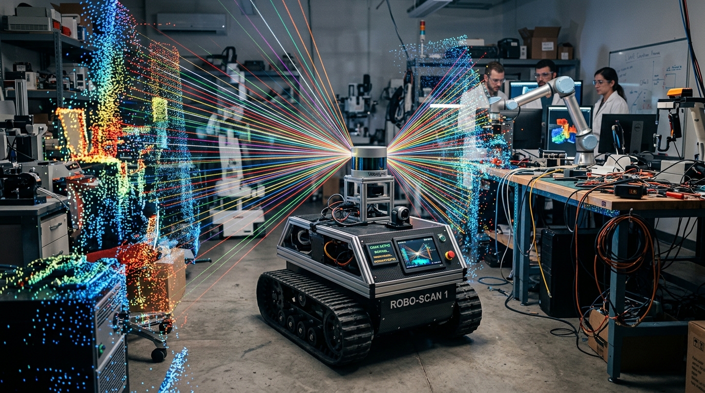
LiDAR Sensors & 3D Point Cloud Processing: ToF Physics, PCL, Voxel Grids & ICP | Knowledge Hub

Core Engineering Takeaways

•Direct Time-of-Flight (dToF) calculates distance from round-trip photon transit time $d = \frac{c \cdot \Delta t}{2}$, requiring picosecond time-to-digital converters.
•Mechanical spinning LiDARs provide uniform 360° field of view, while solid-state MEMS mirror LiDARs provide high reliability without vibrating moving parts.
•Raw point clouds contain 300,000+ points per second; Voxel Grid downsampling is mandatory to condense millions of raw coordinates into uniform volumetric centroids.
•RANSAC (Random Sample Consensus) reliably isolates the ground floor in under 10 ms so robots do not treat the floor as an obstacle.
•Iterative Closest Point (ICP) minimizes Euclidean distance between corresponding point pairs in consecutive scans, providing laser odometry drift rates below 1%.

Prerequisites

Linear algebra (3D rotation matrices, translation vectors, homogeneous coordinates)
Basic probability and statistical outlier modeling
C++ or Python programming fundamentals

1. Ranging Physics: Direct Time-of-Flight vs FMCW Coherent Ranging

LiDAR (Light Detection and Ranging) fires pulsed laser diodes (typically 905 nm or 1550 nm infrared wavelengths) and records reflected photons using high-sensitivity Avalanche Photodiodes (APD) or Single-Photon Avalanche Diodes (SPAD).

Direct Time-of-Flight (dToF)

A laser diode emits a pulse lasting 3 to 10 nanoseconds. The receiver measures time elapsed $\Delta t$ until the reflected photon bundle returns:

d = \frac{c \cdot \Delta t}{2}

Because light travels 30 cm in 1 nanosecond, resolving a 1.5 cm distance requires a time-to-digital converter (TDC) with 100 picosecond accuracy.

Frequency Modulated Continuous Wave (FMCW)

Advanced automotive LiDARs emit continuous laser light with a frequency sweep (chirp). When the reflection returns, it mixes with the local oscillator laser, creating a beat frequency $\Delta f$ . FMCW measures both instantaneous distance and radial Doppler velocity simultaneously without requiring multiple frames.

Direct Time-of-Flight Distance Formula

d = \frac{c \cdot \Delta t}{2 \cdot n_{air}}

In Simple Words: Distance equals speed of light c multiplied by elapsed round-trip flight time Delta t, halved and corrected for refractive index of air.

Variables Breakdown:

d

Distance to reflecting surface targetUnit: Meters (m)

c

Speed of light in vacuum (299,792,458 m/s)Unit: m/s

\Delta t

Measured round-trip time between pulse emission and photodiode detectionUnit: Seconds (s)

n_{air}

Refractive index of ambient air (~1.00029)Unit: Dimensionless

2. LiDAR Hardware Topologies: Mechanical, Multi-Beam & Solid-State MEMS

Different mobile robots require different optical scanning architectures:

1
2D Single-Beam Spinning Mirror (e.g. RPLiDAR, Hokuyo, SICK):

A single laser diode bounces off a rotating mirror spinning at 10 Hz.
Yields a planar 2D slice ( $x, y$ coordinates). Inexpensive ( $100–$ 1,000) and standard for 2D floor SLAM.

2
3D Multi-Beam Mechanical (e.g. Velodyne Puck, Ouster OS1):

Contains 16, 32, 64, or 128 vertical laser emitters spun 360° by an internal brushless motor.
Provides rich vertical angular resolution, but mechanical bearings wear down over years of continuous road vibration.

3
Solid-State MEMS & Flash LiDAR:

Uses microscopic tilting silicon mirrors (MEMS) or flood-illuminates the entire scene with an array of SPAD receivers (Flash LiDAR).
Zero external moving parts, compact automotive integration, but typically restricted to a forward field of view (e.g. 120° × 30°).

Table 1: Comparison of Robotics LiDAR Hardware Classes

LiDAR Class	Field of View (FOV)	Points / Sec	Typical Range	Best Used For
2D Planar Rotating	360° Horizontal x 0° Vertical	5,000 – 16,000	12 – 25 m	Indoor vacuum bots, 2D SLAM warehouse AGVs
3D Multi-Beam Mechanical	360° Horizontal x 30–45° Vertical	300,000 – 2,600,000	50 – 150 m	Off-road rovers, mining trucks, research AMRs
Solid-State MEMS	120° Horizontal x 25° Vertical	500,000 – 1,500,000	150 – 250 m	Autonomous highway cars, forward blind-spot detection
Flash 3D ToF (Solid-State)	90° Horizontal x 65° Vertical	300,000 – 1,000,000	5 – 10 m	Drones, close-range collision avoidance, robot arms

3. Anatomy of a Point Cloud: XYZ, Intensity, Ring & Timestamps

A raw point cloud message in ROS 2 (sensor_msgs/msg/PointCloud2) is a binary serialized byte buffer representing an unordered set of spatial measurements:

X, Y, Z (float32): Cartesian spatial coordinates in meters relative to the sensor frame (lidar_link).
Intensity / Reflectivity (uint8 or float32): Amplitude of the returned laser pulse. High-reflectivity objects (retro-reflective license plates, road tape) return high intensity; dark tires or matte black paint return low intensity.
Ring / Channel (uint16): Which specific physical laser beam produced this measurement (crucial for ground-extraction algorithms).
Timestamp (uint32): Exact nanosecond offset of each pulse, used to de-skew point clouds when the robot is moving at high speed.

Motion Distortion (Motion Skewing)

Because a mechanical LiDAR takes 100 ms to complete a 360° spin, if a robot drives forward at 2 m/s while scanning, the first beam and the last beam are measured 20 cm apart! Always use high-rate IMU interpolation to de-skew raw point clouds before running SLAM.

4. Essential PCL Filtering: PassThrough, Voxel Grid & Statistical Outlier Removal

Processing 1,000,000 raw points per second overwhelms mobile compute. Production robotics utilizes a standardized Point Cloud Library (PCL) pipeline:

1. PassThrough Filter

Cuts off points outside regions of interest (e.g. discard points behind the robot or above 2.5 meters ceiling height).

2. Voxel Grid Downsampling

Divides 3D space into uniform cubic voxels of size $s$ (e.g. $0.05 \text{ m} = 5 \text{ cm}$ ). All points falling within a voxel are averaged into a single centroid. This dramatically reduces point density while preserving geometric structure.

3. Statistical Outlier Removal (SOR)

Removes sensor noise (dust, snow, rain, laser multipath reflections). Computes mean distance $d_i$ from each point to its $k$ nearest neighbors. Points whose mean distance exceeds $\mu + \alpha \cdot \sigma$ are pruned.

voxel_grid_filter.cpp

cpp

#include <pcl/point_types.h>
#include <pcl/filters/voxel_grid.h>
#include <pcl/filters/statistical_outlier_removal.h>

pcl::PointCloud<pcl::PointXYZ>::Ptr filterCloud(pcl::PointCloud<pcl::PointXYZ>::Ptr input_cloud) {
    // 1. Voxel Grid Downsampling (5 cm leaf size)
    pcl::PointCloud<pcl::PointXYZ>::Ptr voxel_filtered(new pcl::PointCloud<pcl::PointXYZ>);
    pcl::VoxelGrid<pcl::PointXYZ> vox;
    vox.setInputCloud(input_cloud);
    vox.setLeafSize(0.05f, 0.05f, 0.05f); // 50mm grid
    vox.filter(*voxel_filtered);

    // 2. Statistical Outlier Removal
    pcl::PointCloud<pcl::PointXYZ>::Ptr sor_filtered(new pcl::PointCloud<pcl::PointXYZ>);
    pcl::StatisticalOutlierRemoval<pcl::PointXYZ> sor;
    sor.setInputCloud(voxel_filtered);
    sor.setMeanK(20);             // Analyze 20 nearest neighbors
    sor.setStddevMulThresh(1.0);  // Reject points > 1.0 standard deviation from mean
    sor.filter(*sor_filtered);

    return sor_filtered;
}

Note: Standard C++ PCL filter pipeline converting high-noise raw laser scans into clean, uniform point representations ready for registration and mapping.

5. Segmentation: RANSAC Ground Plane Removal & Euclidean Clustering

Before a mobile robot can detect pedestrians or obstacles, it must remove the road surface from the point cloud.

RANSAC Ground Plane Extraction

A flat ground surface satisfies the planar equation:

a x + b y + c z + d = 0

RANSAC (Random Sample Consensus) randomly selects 3 points, fits a candidate plane, and counts inlier points within distance threshold $\epsilon$ (e.g., 5 cm). After 50 iterations, the model with the highest inliers is extracted as ground and subtracted from the scene.

Euclidean Cluster Extraction

Once the ground plane is removed, remaining points are grouped into distinct obstacle clusters (cars, humans, walls) using KD-Tree nearest neighbor queries with a distance tolerance (e.g., 30 cm).

Point-to-Plane Euclidean Distance Formula

D_{plane}(p) = \frac{|a x_p + b y_p + c z_p + d|}{\sqrt{a^2 + b^2 + c^2}}

In Simple Words: Calculates the perpendicular distance from 3D point p to candidate plane coefficients (a, b, c, d) during RANSAC iterations.

Variables Breakdown:

D_{plane}(p)

Orthogonal distance from point p to the candidate planeUnit: Meters

(x_p, y_p, z_p)

Coordinates of point in the sensor point cloudUnit: Meters

(a, b, c)

Normal vector coordinates of the candidate ground planeUnit: Dimensionless

d

Offset distance of the plane from the coordinate originUnit: Meters

6. Point Cloud Alignment: Iterative Closest Point (ICP) & NDT

How does a robot know how far it traveled between two laser scans? By matching consecutive 3D point clouds!

Iterative Closest Point (ICP)

1
For each point $p_i$ in the current scan, find the closest point $q_i$ in the reference scan.
2
Compute the optimal 3D rigid transform $[R | t]$ minimizing the sum of squared distances:

E(R, t) = \sum_{i=1}^{N} \| R p_i + t - q_i \|^2

3
Transform the current scan by $[R | t]$ and repeat until convergence.

Normal Distributions Transform (NDT)

Rather than matching individual points, NDT divides space into cells and fits a 3D Gaussian probability distribution to each cell. NDT converges significantly faster than ICP on sparse automotive LiDAR scans.

Table 2: Scan Matching Algorithms in 3D SLAM

Algorithm	Data Representation	Convergence Speed	Sensitivity to Initialization	Best Use Case
Point-to-Point ICP	Raw Point Coordinates	Slow	High (Requires good initial guess)	Dense indoor RGB-D room scans
Point-to-Plane ICP	Point with Surface Normals	Fast (Fewer iterations)	Moderate	Structured indoor environments with walls
NDT (Normal Distributions)	3D Gaussian Probability Grids	Very Fast	Low / Robust	Outdoor highway and high-speed autonomous driving
GICP (Generalized ICP)	Plane-to-Plane Covariance	Moderate-Fast	Moderate	High-accuracy survey mapping and geodesy

Frequently Asked Questions

Common Questions & Troubleshooting

Q:Why does LiDAR struggle with glass windows and black matte cars?

Standard 905nm infrared laser light passes directly through clear glass (specular transmission), producing either no return or measuring objects behind the window! Glossy or black matte surfaces absorb laser photons or reflect them away at sharp angles (specular reflection), causing point dropouts. Robots counter this by combining LiDAR with ultrasonic sensors (which bounce off glass) and stereo vision.

Q:What is the advantage of 1550 nm LiDAR over 905 nm LiDAR?

905 nm laser light passes into human eyes and can burn retinas, so emitter power is strictly limited by eye-safety regulations. 1550 nm light is absorbed in the eye cornea before reaching the retina, allowing manufacturers to emit up to 40x higher laser power without violating eye-safety rules, enabling ranges of 250+ meters in rain and fog.

Q:What leaf size should I choose for Voxel Grid filtering?

For indoor differential drive robots navigating offices, 0.03 m to 0.05 m (3 to 5 cm) provides an ideal balance of detail and CPU speed. For outdoor autonomous vehicles operating at 30-50 km/h, use 0.10 m to 0.20 m (10 to 20 cm) leaf sizes to sustain 20 Hz real-time SLAM.

Previous ArticleAutonomous Navigation & Path Planning: Global, Local Planners & Nav2 Costmaps Explained Next ArticleRobot Simulation & Digital Twins: Gazebo Harmonic, NVIDIA Isaac Sim, URDF & Physics Engines